Assignment #2 - Gradient Domain Fusion

Award Winners!

We’ve completed the homework, grading, and voting, and the winner of our best assignment is Riyaz Panjwani!

Honorable Mentions go to Tomas Cabezon Pedroso and Harry Freeman. Great work to all and check out the winning projects!

Background

This project explores gradient-domain processing, a simple technique with a broad set of applications including blending, tone-mapping, and non-photorealistic rendering. For the core project, we will focus on “Poisson blending”; tone-mapping and NPR can be investigated as bells and whistles.

The primary goal of this assignment is to seamlessly blend an object or texture from a source image into a target image. The simplest method would be to just copy and paste the pixels from one image directly into the other. Unfortunately, this will create very noticeable seams, even if the backgrounds are well-matched. How can we get rid of these seams without doing too much perceptual damage to the source region?`

Here we take the following approach: The insight we will use is that people often care much more about the gradient of an image than the overall intensity. So we can set up the problem as finding values for the target pixels that maximally preserve the gradient of the source region without changing any of the background pixels. Note that we are making a deliberate decision here to ignore the overall intensity! So a green hat could turn red, but it will still look like a hat.

We can formulate our objective as a least squares problem. Given the pixel intensities of the source image “s” and of the target image “t”, we want to solve for new intensity values “v” within the source region “S”:

\(\newcommand{\argmin}{arg min}\) \(\boldsymbol{v} = \argmin_{\boldsymbol{v}}\sum_{i \in S, j \in N_i \cap S}((v_i - v_j) - (s_i - s_j))^2 + \sum_{i\in S, j \in N_i \cap \neg S}((v_i - t_j) - (s_i - s_j))^2.\)

Here, each “i” is a pixel in the source region “S”, and each “j” is a 4-neighbor of “i”. Each summation guides the gradient values to match those of the source region. In the first summation, the gradient is over two variable pixels; in the second, one pixel is variable and one is in the fixed target region.

The method presented above is called “Poisson blending”. Check out the Perez et al. 2003 paper to see sample results, or to wallow in extraneous math. This is just one example of a more general set of gradient-domain processing techniques. The general idea is to create an image by solving for specified pixel intensities and gradients.

A Wordy Explanation

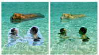
As an example, consider this picture of the bear and swimmers being pasted into a pool of water. Let’s ignore the bear for a moment and consider the swimmers. In the above notation, the source image “s” is the original image the swimmers were cut out of; that image isn’t even shown, because we are only interested in the cut-out of the swimmers, i.e., the region “S”. “S” includes the swimmers and a bit of light blue background. You can clearly see the region “S” in the left image, as the cutout blends very poorly into the pool of water. The pool of water, before things were rudely pasted into it, is the target image “t”.

So, how do we blend in the swimmers? We construct a new image “v” whose gradients inside the region “S” are similar to the gradients of the cutout we’re trying to paste in (swimmers + a little bit of background). The gradients won’t end up matching exactly: the least squares solver will take any hard edges of the cutout at the boundary and smooth them by spreading the error over the gradients inside “S”.

Outside “S”, “v” will match the pool. We won’t even bother computing the gradients of the pool outside S; we’ll just copy those pixels directly.

In the first half of the large equation above, we set the gradients of “v” inside S. We loop over all the pixels inside the region S, and request that our new image “v” have the same gradients as the swimmers. The summation is over every pixel i in S; j is the 4 neighbors of i (left, right, up, and down, giving us both the x and y gradients. You may notice this equation counts all the gradients twice - is was simpler to write it this way. You actually don’t have to double-count everything; it doesn’t affect the result.)

But what do we do around the boundary of “S”? I.e. what if i is inside S, but j is outside? That’s the second half of the equation. (If you look closely at the variables under the summation sign, the S has a bar thing in front of it - that means the complement of S, or anything not in S. Thus, read “j in the 4-neighborhood of i, but j not in S”). In this case we aren’t solving for a v_j, since j is not inside “S”. So we just pluck the intensity value right out of the target image. Thus we use t_j. Remember, we aren’t modifying t outside the area of S, so we know that v_j in this case isn’t a variable: it’s exactly equal to t_j.

Part 1.1 Toy Problem (20 pts)

The implementation for gradient domain processing is not complicated, but it is easy to make a mistake, so let’s start with a toy example. In this example we’ll compute the x and y gradients from an image s, then use all the gradients, plus one pixel intensity, to reconstruct an image v.

Denote the intensity of the source image at (x, y) as s(x,y) and the values of the image to solve for as v(x,y). For each pixel, then, we have two objectives:

1. Minimize \((( v(x+1,y)-v(x,y)) - (s(x+1,y)-s(x,y)) )^2\), so the x-gradients of v should closely match the x-gradients of s.
2. Minimize \((( v(x,y+1)-v(x,y)) - (s(x,y+1)-s(x,y)) )^2\), so the y-gradients of v should closely match the x-gradients of s. Note that these could be solved while adding any constant value to v, so we will add one more objective:

3. minimize \((v(1,1)-s(1,1))^2\)

   The top left corners of the two images should be the same color

For 20 points, solve this optimization as a least squares problem. If your solution is correct, then you should recover the original image.

Implementation Details

(The implement details below is served more as a pseudocode. You might find yourself constructing a matrix in a slightly different way because a sparse matrix might need to be instantiated differently. However, the details below should give you an accurate mental picture of how you would like to implement your algorithm.)

The first step is to write the objective function as a set of least squares constraints in the standard matrix form: (Av-b)^2. Here, “A” is a sparse matrix, “v” are the variables to be solved, and “b” is a known vector. It is helpful to keep a matrix “im2var” that maps each pixel to a variable number, such as:

imh, imw, nb = im.shape
im2var = np.arange(imh * imw).reshape((imh, imw)).astype(int)

(If you find that trick confusing, understand that you could have performed the mapping between pixel and variable number manually each time: e.g. the pixel at s(r,c), uses the variable number (c-1)*imh+r. However, this trick will come in handy for Poisson blending, where the mapping is from an arbitrarily-shaped block of pixels and won’t be such a simple function. So it makes sense to understand it now.)

Then, you can write Objective 1 above as:

e += 1
A[e, im2var[y, x + 1]] = 1
A[e, im2var[y, x] = -1
b[e] = s[y, x + 1] - s[y, x]

Here, “e” is used as an equation counter. Note that the y-coordinate is the first index as we’re assuming row-major images. Objective 2 is similar; add all the y-gradient constraints as more rows to the same matrices A and b.

As another example, Objective 3 above can be written as:

e += 1
A[e, im2var[0, 0]] = 1
b[e] = s[0, 0]

To solve for v, use numpy’s linear algebra solving capabilities, such as lstsq or solve in the np.linalg package.

Then, copy each solved value to the appropriate pixel in the output image.

Part 1.2 Poisson Blending (60 pts)

Step 1: Select source and target regions. Select the boundaries of a region in the source image and specify a location in the target image where it should be blended. Then, transform (e.g., translate) the source image so that indices of pixels in the source and target regions correspond. We’ve provided starter code that will help with this. You may want to augment the code to allow rotation or resizing into the target region. You can be a bit sloppy about selecting the source region – just make sure that the entire object is contained. Ideally, the background of the object in the source region and the surrounding area of the target region will be of similar color.

Step 2: Solve the blending constraints.

Step 3: Copy the solved values v_i into your target image. For RGB images, process each channel separately. Show at least three results of Poisson blending. Explain any failure cases (e.g., weird colors, blurred boundaries, etc.).

Tips

1. For your first blending example, try something that you know should work, such as the included penguins on top of the snow in the hiking image.
2. Object region selection can be done very crudely, with lots of room around the object.

Bells & Whistles (Extra Points)

Mixed Gradients (5 pts)

Follow the same steps as Poisson blending, but use the gradient in source or target with the larger magnitude as the guide, rather than the source gradient: \(\boldsymbol{v} = \argmin_{\boldsymbol{v}} \sum_{i \in S, j \in N_i \cap S} ((v_i - v_j) - d_{ij})^2 + \sum_{i \in S, j \in N_i \cap \neg S}((v_i - t_j) - d_{ij})^2.\) Here “\(d_{ij}\)” is the value of the gradient from the source or the target image with larger magnitude, i.e.

if abs(s_i - s_j) >= abs (t_i - t_j):
    d_ij = s_i - s_j
else:
    d_ij = t_i - t_j

Show at least one result of blending using mixed gradients. One possibility is to blend a picture of writing on a plain background onto another image.

Color2Gray (2 pts)

Sometimes, in converting a color image to grayscale (e.g., when printing to a laser printer), we lose the important contrast information, making the image difficult to understand. For example, compare the color version of the image on right with its grayscale version produced by MATLAB’s rgb2gray.

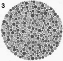
Can you do better than rgb2gray? Gradient-domain processing provides one avenue: create a gray image that has similar intensity to the rgb2gray output but has simoilar contrast to the original RGB image. This is an example of a tone-mapping problem, conceptually similar to that of converting HDR images to RGB displays. To get credit for this, show the grayscale image that you produce (the numbers should be easily readable).

Hint: Try converting the image to HSV space and looking at the gradients in each channel. Then, approach it as a mixed gradients problem where you also want to preserve the grayscale intensity.

More gradient domain processing (up to 3 pts)

Many other applications are possible, including non-photorealistic rendering, edge enhancement, and texture or color transfer. See Perez et al. 2003 and GradientShop for further ideas.

Grading

This assignment will be graded out of 100 points, as follows:

• (20 points) Include a brief description of the project
• (20 points) Finish the toy problem.
• (35 points) Show your favorite blending result. Include: 1) the source and target image; 2) the blended image with the source pixels directly copied into the target region; 3) the final blend result. Briefly explain how it works, along with anything special that you did or tried. This should be with your own images, not the included samples.
• (25 points) Next, show at least two more results for Poisson blending, including one that doesn’t work so well (failure example). Explain any difficulties and possible reasons for bad results.

Some Hints

• You may use scipy.sparse for large sparse matrix computation.
• You might find scipy.sparse.linalg.lsqr helpful.
• Pay attention to the image intensity scale. Sometimes the bug is in the visualization even though the algorithm is right.
• Pay attention to the boundary condition.

Materials

• Starter Code and Images, including a top-level script (proj2_starter.py) and functions (masking_code.py, README.md) to select the source region and align source and target images for blending.

Acknowledgement: The assignment is credit to Berkeley CS194-26. The hybrid images part of the assignment is borrowed from Derek Hoiem’s Computational Photography class. The gradient domain part of this assigment was based on one offered by Derek Hoiem and has also been written up by James Hays.